Bench Inspection Day!

Finally, the time has come, where all our hard work spent on the project is showcased for all to see. In the form of a poster, lab book and this blog (along with a few real time practical simulations), we present our findings of how DSSS in 3G communications is possible. Our main focus with this project was the CDMA modulation technique, which is widely used in industry. Without this modulation technique it would be difficult to transmit the Data securely and efficiently.

A lot has been learnt about how Matlab can be used to simulate physical systems, which can be vital in helping with the design process and to ensure the system works before implementing it. 

In the 6 weeks we have been given to produce a project, it has been difficult at times but I think the results we have obtained have been significant in showing how a DSSS system functions.

CDMA code for 4 Users

The text below is the final code a simulation that can extract the original data of 4 separate users from the interference pattern of 64 simultaneous users. This is code was used for the previous post.

%This script runs a simulation of a 64 simultaneous user system where 4 
%users need to be extracted by using their unique spreading code. The
%script then plots graphs of original data, the spreading code for each of
%the 4 users, the interference pattern and the recovered signal. All
%contained within a figure.


%Declares the variables
Length =20;
Users =64; 
Index1 =7;
Index2 =20;
Index3 =30;
Index4 =43;
spread = 0;
V = [1,-1];
L = Users * Length;
%Generates a random noise pattern
noise =  V(randi([1,numel(V)],L,1));

W = [1];

%A loop that generates the Walsh-Hadamard matrix.
for n = 1 : log2(Users);
    W = [ W W ; W -W];
end

%A loop that spreads user signal with spreading code unique to each user
%and then combines the spreading signals of each user into an interference
%pattern
for x=0 : (Users-1);

    %Generates spreading code for each user based on their user number.
    code = W(x+1, :);

    %Generates a random set of data for each user to transmit.
    D1 = UserData(Length);

    %This will multiply the spreading code by individual bit of User Data.
    spread1=[code*D1(1),code*D1(2),code*D1(3),code*D1(4),code*D1(5),code*D1(6),code*D1(7),code*D1(8),code*D1(9),code*D1(10),code*D1(11),code*D1(12),code*D1(13),code*D1(14),code*D1(15),code*D1(16),code*D1(17),code*D1(18),code*D1(19),code*D1(20)];

    %Checks for user one.
    if x == Index1
        UserD1 = D1; 
        SpreadC1 = code;
    end
    %Checks for user two.
      if x == Index2
                UserD2 = D1;
                SpreadC2 = code;
      end 
      %Checks for user three.
           if x == Index3
                    UserD3 = D1;  
                    SpreadC3 = code;
           end     
           %Checks for user four.
               if x == Index4
                        UserD4 = D1; 
                        SpreadC4 = code;
               end

    %Adds spread signal to the interference pattern after each loop.           
    spread=spread+spread1;     
end

%Adds noise to the interference pattern.
spread=spread+noise

%Extracts the two pieces of user data from the interference pattern.
c1=despread(SpreadC1,spread);
c2=despread(SpreadC2,spread);
c3=despread(SpreadC3,spread);
c4=despread(SpreadC4,spread);

%These all declare the axis for the graphs.
Plot1X1=size(UserD1);
X1= [1:(Plot1X1(2))];

Plot1X2=size(UserD2);
X2= [1:(Plot1X2(2))];

Plot1X3=size(UserD3);
X3= [1:(Plot1X3(2))];

Plot1X4=size(UserD4);
X4= [1:(Plot1X4(2))];

Plot3X1=size(SpreadC1);
Plot3X1=Plot3X1(1)*Plot3X1(2);
X5= [1:(Plot3X1)];

Plot3X2=size(SpreadC2);
Plot3X2=Plot3X2(1)*Plot3X2(2);
X6= [1:(Plot3X2)];

Plot3X3=size(SpreadC3);
Plot3X3=Plot3X3(1)*Plot3X3(2);
X7= [1:(Plot3X3)];

Plot3X4=size(SpreadC4);
Plot3X4=Plot3X4(1)*Plot3X4(2);
X8= [1:(Plot3X4)];

Plot5X1=size(spread);
Plot5X1=Plot5X1(1)*Plot5X1(2);
X9= [1:(Plot5X1)];

Plot7X1=length(c1);
X10=[1:Plot7X1];

Plot7X2=length(c2);
X11=[1:Plot7X2];

Plot7X3=length(c3);
X12=[1:Plot7X3];

Plot7X4=length(c4);
X13=[1:Plot7X4];


%The following code plots 13 graphs in the form of a square wave plotted in 
%a single figure.
h1=subplot(5,4,1);plot(X1,UserD1)
h1=stairs(X1,UserD1);
grid 'on';
title('Data set 1 to be transmitted.')

h2=subplot(5,4,2);plot(X2,UserD2)
h2=stairs(X2,UserD2);
grid 'on';
title('Data set 2 to be transmitted.')

h3=subplot(5,4,3);plot(X3,UserD3)
h3=stairs(X3,UserD3);
grid 'on';
title('Data set 3 to be transmitted.')

h4=subplot(5,4,4);plot(X4,UserD4)
h4=stairs(X4,UserD4);
grid 'on';
title('Data set 4 to be transmitted.')

h5=subplot(5,4,5:6);plot(X5,SpreadC1)
h5=stairs(X5,SpreadC1);
grid 'on';
title('Spread data 1.')

h6=subplot(5,4,7:8);plot(X6,SpreadC2)
h6=stairs(X6,SpreadC2);
grid 'on';
title('Spread data 2.')

h7=subplot(5,4,9:10);plot(X7,SpreadC3)
h7=stairs(X7,SpreadC3);
grid 'on';
title('Spread data 3.')

h8=subplot(5,4,11:12);plot(X8,SpreadC4)
h8=stairs(X8,SpreadC4);
grid 'on';
title('Spread data 4.')

h9=subplot(5,4,13:16);plot(X9,spread)
h9=stairs(X9,spread);
grid 'on';
title('Transmitted signal including interference')

h10=subplot(5,4,17);plot(X10,c1)
h10=stairs(X10,c1);
grid 'on';
title('Despread Signal 1')

h11=subplot(5,4,18);plot(X11,c2)
h11=stairs(X11,c2);
grid 'on';
title('Despread Signal 2')

h12=subplot(5,4,19);plot(X12,c3)
h12=stairs(X12,c3);
grid 'on';
title('Despread Signal 3')

h13=subplot(5,4,20);plot(X13,c4)
h13=stairs(X13,c4);
grid 'on';
title('Despread Signal 4')

Clean system versus noise added system

The system above is clean (without added noise). This just shows that at least 4 different users can be extracted from the interference pattern comprised of 64 unique spread signals. Its important to test if the system is capable of spreading and despreading the signal before integrity testing can be done. Each signal is colour coordinated with their spreading signal and despread data code, making the evaluation easier.



The same users would like to transmit a different set of data, but this time the system is being affected by some form of noise. The noise used was a random 1 & -1 sequence with the same length as the interference pattern and added to it before the data is despread. The data does keep its original shape however it has a slightly distorted to it but only slightly and as we have noticed, the same noise becomes less effective as the length of the spreading code increases, which boasts improved performance.

Meet the Team Working Hard

On the left is Matthew Davies. He is currently showing of one of his new poses, which he will be using in his new modelling job "Just For Gingers" magazine. Whilst apparently working.













On the right is Hamish Smellie, with his unprecedented 'knowledge' of 3G communication. Currently sporting the hard working student look, his body language shows he is uncomfortable with this.

Hadamard Sequence

There is a very simple way to create a set Hadamard codes, it is called the the recursive technique.

Below is an example of how four sequences of code are created from the two sets using the above formula.

So above shows four sequences of code and three lines of code are used for characteristics, synchronization and paging. Which means that a four chip spreading code, like above, will only have one available slot for a user.

Synchronization of Spread Spectrum Signals

For the reciever to be able to demodulate the recived signal, the reciever clock and the transmitter clock need to be in sync. So this is why the reciver clock and the transmitter clock are extremely stable and accurate. This would work well if the reciver was right next to the transmitter, but in most cases they are not very close at all. Therefore there is a time uncertainty.

This is the formual for the time delay, where N is the number of chips in the spreading code and Tc is the time taken for on chip.
So if we were to search over the time uncertainty inerval in time steps of 1/2Tc, then the time required to establish initial synchronization is:

Testing with multiple users

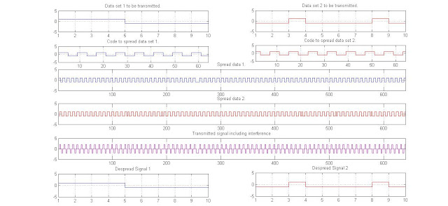
Here we have the results of using 2 separate users with different spreading codes and data. The blue coloured plot represents the components for User 1 and the red coloured plots represent the components for User 2. The combined spread signal or 'interference pattern' is purple. The basic method of receiving the original data from the interference pattern is to multiply the pattern with the original spreading code, and then divide the signal by however many users are in the interference signal.

Walsh code spreading

The figure to the left shows how the Walsh code is multiplied with the data to give a spread signal with a higher frequency. The Walsh code and the data were both created using Matlab along with the plotted graphs.  

Pseudo Noise

Pseudo Noise is an important feature of modulating data that is transmitted wirelessly. Also known as Pseudo Random code, it is a sequence of numbers that look random, but can be recreated relatively easily.

The pseudo noise is generated using an algorithm based on inputted numbers and this 'noise' is multiplied with the data that needs to be transmitted to produce a 'spreaded' version of the signal. The spreading of the signal usually transforms the signal into one that is below the natural noise level. This makes the signal hard to trace and intercept or scramble.

Spread Signal below noise level

The pseudo noise is unique to each user, so that users can transmit and receive data simultaneously without the user receiving the wrong data or the data of one user transforming with another because the have the same spreading code (pseudo noise code).

There are a few pseudo noise techniques that are used for CDMA, such as; Gold Codes, Walsh- Hadamard Code, M-Sequence Code, Barker Code and Kasami Code.

We will be focussing mainly on Walsh- Hadamard Code and M-Sequence Code.